Control#

The Controller of the MPMCA is a Non-Linear Model Predictive Controller that calculates the control inputs to be provided to the simulator (or: controlled system, plant) in order to follow the reference output as optimally as possible (governed by a cost function) whilst making sure that the system stays within the provided constraints. These pages will provide more precise mathematical definitions of the cost function that is optimized, the equations governing the system behavior, the output functions, and the constraint functions. \( \newcommand{\Dtmpc}{{\Delta t}} \newcommand{\Fx}{{f_x}} \newcommand{\Fy}{{f_y}} \newcommand{\Fz}{{f_z}} \newcommand{\RefInput}{\hat{\Input}} \newcommand{\RefState}{\hat{\State}} \newcommand{\RefOutput}{\skew{3}\hat{\Output}} \newcommand{\RefOutputScalar}{\skew{3}\hat{\OutputScalar}} \newcommand{\RefSpecForce}{\SpecForceRef} \newcommand{\RefW}{\hat{\RotVel}} \newcommand{\RefWx}{{\hat{\omega}_x}} \newcommand{\RefWy}{{\hat{\omega}_y}} \newcommand{\RefWz}{{\hat{\omega}_z}} \newcommand{\Input}{\mathbf{u}} \newcommand{\State}{\mathbf{x}} \newcommand{\WState}{\boldsymbol{W}_\State} \newcommand{\WInput}{\boldsymbol{W}_\Input} \newcommand{\WOutput}{\boldsymbol{W}_\Output} \newcommand{\Ax}{{\alpha_x}} \newcommand{\Ay}{{\alpha_y}} \newcommand{\Az}{{\alpha_z}} \newcommand{\ErrAx}{{\tilde{\alpha}_x}} \newcommand{\ErrAy}{{\tilde{\alpha}_y}} \newcommand{\ErrAz}{{\tilde{\alpha}_z}} \newcommand{\ErrFx}{{\tilde{f}_x}} \newcommand{\ErrFy}{{\tilde{f}_y}} \newcommand{\ErrFz}{{\tilde{f}_z}} \newcommand{\ErrWx}{{\tilde{\omega}_x}} \newcommand{\ErrWy}{{\tilde{\omega}_y}} \newcommand{\ErrWz}{{\tilde{\omega}_z}} \newcommand{\ExpAx}{{\Ax^{\mathrm{p}}}} \newcommand{\ExpAy}{{\Ay^{\mathrm{p}}}} \newcommand{\ExpAz}{{\Az^{\mathrm{p}}}} \newcommand{\ExpF}{\SpecForce^{\mathrm{p}}} \newcommand{\ExpFx}{{\Fx^{\mathrm{p}}}} \newcommand{\ExpFy}{{\Fy^{\mathrm{p}}}} \newcommand{\ExpFz}{{\Fz^{\mathrm{p}}}} \newcommand{\ExpOutput}{\Output^\mathrm{p}} \newcommand{\ExpState}{\State^\mathrm{p}} \newcommand{\ExpInput}{\Input^\mathrm{p}} \newcommand{\ExpRotVel}{\RotVel^{\mathrm{p}}} \newcommand{\ExpSpecForce}{\SpecForceExp} \newcommand{\Output}{\boldsymbol{y}} \newcommand{\ActOutput}{\Output^\mathrm{a}} \newcommand{\ActState}{\State^\mathrm{a}} \newcommand{\ActInput}{\Input^\mathrm{a}} \newcommand{\F}{\SpecForce} \newcommand{\A}{\RotAcc} \newcommand{\RefA}{\hat{\RotAcc}} \newcommand{\RotVel}{\boldsymbol{\omega}} \newcommand{\W}{\RotVel} \newcommand{\SpecForce}{\boldsymbol{f}} \newcommand{\RotAcc}{\boldsymbol{\alpha}} \newcommand{\A}{\RotAcc} \newcommand{\RefA}{\hat{\RotAcc}} \newcommand{\Wx}{{\omega_x}} \newcommand{\Wy}{{\omega_y}} \newcommand{\Wz}{{\omega_z}} \newcommand{\Wyax}{{W_{\Ax}}} \newcommand{\Wyay}{{W_{\Ay}}} \newcommand{\Wyaz}{{W_{\Az}}} \newcommand{\Wyfx}{{W_{\Fx}}} \newcommand{\Wyfy}{{W_{\Fy}}} \newcommand{\Wyfz}{{W_{\Fz}}} \newcommand{\Wywx}{{W_{\Wx}}} \newcommand{\Wywy}{{W_{\Wy}}} \newcommand{\Wywz}{{W_{\Wz}}} \)

Cost function#

At every control interval, the Controller finds a simulator trajectory for which the cost function, defined as:

\(J = \displaystyle \frac{1}{N} \sum_{k=0}^{N-1} \left( \left\Vert\ExpOutput(\ExpState_k,\ExpInput_k) - {\RefOutput}_k \right\Vert_{\WOutput}^2 + \left\Vert \ExpState_k-{\RefState}_k\right\Vert_{\WState}^2 + \left\Vert \ExpInput_k-\RefInput_k\right\Vert_{\WInput}^2 \right) \Dtmpc_k\)

is minimum, with \(\ExpInput_k\) the planned input to be given to the system at discrete time steps \(k\), \(\ExpState_k\) the planned state of the system resulting from the planned inputs, \(\ExpOutput\in \mathbb{R}^{9}\) the planned output of the system resulting from the planned states and inputs, \(\hat{\Output}_k\) the predicted reference output signals, \(\hat{\State}_k\) the reference state, \(\hat{\Input}_k\) the reference input, \(\Dtmpc_k\) the duration of the control interval at discrete time step \(k\), and \(N\) the number of samples in the prediction horizon. The symmetric positive-definite weighting matrices \(W_\Output\), \(W_\State\), and \(W_\Input\) determine the relative importance of the three terms.

Output error#

The first term, the output-error term, measures the distance from the predicted reference output to the planned output. When using the MPMCA for motion cueing, the output comprises nine inertial signals measured in the head frame of reference: three specific forces, \(f_x\), \(f_y\), and \(f_z\), three angular velocities \(\omega_x\), \(\omega_y\), and \(\omega_z\), and three angular accelerations \(\alpha_x\), \(\alpha_y\), and \(\alpha_z\). Thus:

\(\Output = \left[\F^{T}~\W^{T}~\A^{T}\right]^{T} = \left[\Fx~\Fy~\Fz~\Wx~\Wy~\Wz~\Ax~\Ay~\Az \right]^{T}\)

Hence, the output error weight matrix is given as:

\(\WOutput = {\rm diag} \left(\left[\Wyfx~\Wyfy~\Wyfz~\Wywx~\Wywy~\Wywz~\Wyax~\Wyay~\Wyaz \right] \right)\)

Note that the methods in the code to set the output error weight take a vector as input, which contains the elements on the diagonal of the matrix only.

Typical values for the output error weight matrix are as follows. These values are an acceptable start for the tuning process:

\(\WOutput = {\rm diag} \left(\left[1~1~1~10~10~10~0.1~0.1~0.1 \right] \right)\)

Note that the MPMCA can also be used to control the pose (position and orientation) of the end-effector of a robot, but this feature is not documented at the moment. Get in touch if you are planning to use this feature!

State error#

The second term in the cost function is referred to as the state-error term and represents the distance of the planned state trajectory to the reference state. The system is pulled towards the reference state \(\RefState_k\) for \(\WState > 0\). The state-error term acts as a form of washout if \(\RefState_k\) represents a state in the center of the motion space with zero velocity. The state of the simulator typically consists of the position and velocity signals of each degree of freedom. For example, the state vector for a 6DOF hexapod simulator is defined as:

\(\State = \left[x~y~z~\phi~\theta~\psi~\dot{x}~\dot{y}~\dot{z}~p~q~r\right]^{T}\)

And so the state error weight matrix is given as:

\(\WState = {\rm diag} \left( \left[W_x~W_{y}~W_{z}~W_{\phi}~W_{\theta}~W_{\psi}~W_{\dot{x}}~W_{\dot{y}}~W_{\dot{z}}~W_{p}~W_{q}~W_{r} \right] \right)\)

Typical values for the state error weight matrix are approximately 1 for the position weight values and close to zero for the velocity weight values.

Input error#

The third term in the cost function is referred to as the input-error term and represents the distance of the planned inputs to the reference input. \(\RefInput_k = \boldsymbol{0}\) and \(W_\Input > 0\) promotes small inputs and improves the local convexity of the optimization problem, which improves convergence speed. The input of the simulator consists of the second derivatives of all position signals.

For example, the input vector for a 6DOF hexapod simulator is defined as:

\(\Input = \left[\ddot{x}~\ddot{y}~\ddot{z}~\dot{p}~\dot{q}~\dot{r}\right]^{T}\)

And so the input error weight matrix is given as:

\(\WInput = \left[W_{\ddot{x}}~W_{\ddot{y}}~W_{\ddot{z}}~W_{\dot{p}}~W_{\dot{q}}~W_{\dot{r}}\right]^{T}\)

Typical values for the input weights are approximately 0.1.

System dynamics and geometry#

The simulators and robotic systems that are part of the MPMCA by default are all modelled as double integrator systems, with position and velocity as states and acceleration as input. The coordinate systems and model descriptions for three simulators are described below:

1. The Constraint Free Simulator (MpmcaConstraintFreeSimulator): a platform moving in all six degrees of freedom without any other constraints than simple box constraints on the states.
2. The Hexapod (MpmcaHexapod): a basic hexapod Stewart platform with six legs.
3. The XY, Hexapod, Yaw Simulator (MpmcaXyHexapodYaw): a hexapod Stewart platform placed onto a XY table and a Yaw table attached to the moving platform of the hexapod.

Detailed documentation on the Industrial Robot systems is not provided yet, but see ¹ for hints.

Constraint Free Simulator#

The relevant coordinate systems and model of the MpmcaConstraintFreeSimulator are shown below. Note that the aircraft frame of reference (\(x\) positive forward, \(y\) postive to the right, and \(z\) positive down) is used.

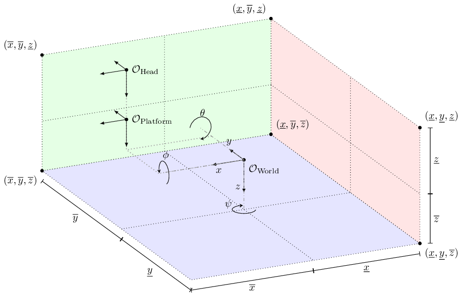
The 'platform' is essentially the point \(\mathcal{O}_{\rm Platform}\) moving through space relative to the world origin at \(\mathcal{O}_{\rm World}\), with linear translations \(x\), \(y\), and \(z\), and Euler angles roll \(\phi\), pitch \(\theta\), and yaw \(\psi\) (rotation order: yaw, pitch, roll). The constraints on each state and input are simply 'box constraints', i.e., the minimum and maximum allowed values. The constraints on the translational degrees of freedom are shown graphically, with the lower bounds denoted by the underbar \(\underline{*}\) and the upper bounds by the overbar \(\overline{*}\). Note that the cueing point at \(\mathcal{O}_{\rm Head}\) is 'fixed to' the platform at \(\mathcal{O}_{\rm Platform}\) (through the final transformation matrix) and does not have its own constraints.

Hexapod#

The coordinate systems and kinematic model of the MpmcaHexapod simulator are shown below. It is similar to the Constraint Free Simulator, but has additional limits imposed by the six legs.

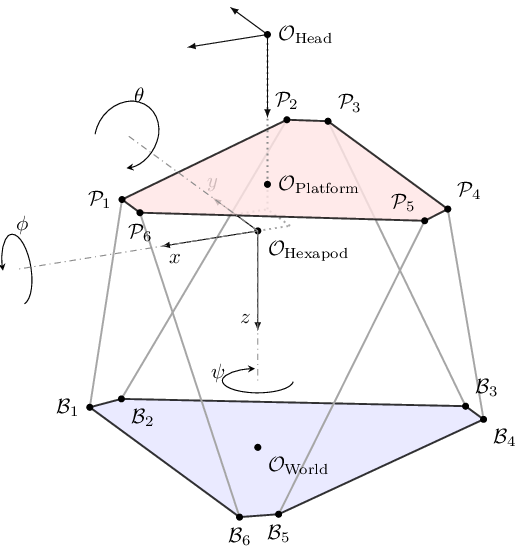
The origin of the hexapod \(\mathcal{O}_{\rm Hexapod}\) is defined by a coordinate transformation with respect to the origin of the world coordinate frame \(\mathcal{O}_{\rm World}\). For the MpmcaHexapod, this is a (negative) translation in the z-direction, to align the platform base joints with the ground level. The origin of the moving platform \(\mathcal{O}_{\rm Platform}\) coincides with \(\mathcal{O}_{\rm Hexapod}\) when the translations \(x\), \(y\), and \(z\) are equal to zero.

The joint coordinates of the moving platform \(\mathcal{P}_{(1,6)}\) and the joint coordinates of the fixed base \(\mathcal{B}_{(1,6)}\) are defined in the Hexapod coordinate frame. Thus, the numerical values of the \(z\) coordinates of \(\mathcal{P}_{(1,6)}\) are typically close to zero, and those of \(\mathcal{B}_{(1,6)}\) are typically much greater than zero. The final transformation matrix defines the transformation from \(\mathcal{O}_{\rm Platform}\) to the 'cueing point' at \(\mathcal{O}_{\rm Head}\), which is typically at the center of the head of the human inside the simulator. Since \(z\) is positive down, the \(z\) translation is typically negative.

Hexapod with yaw table on XY table#

The coordinate system and kinematic model of the MpmcaXyHexapodYaw simulator, which consists of an XY table, a hexapod, and a yaw table, is shown below.

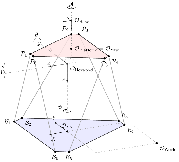
The XY table is simply a coordinate system \(\mathcal{O}_{\rm XY}\) that can move along the \(X\) and \(Y\) axes of the world coordinate system \(\mathcal{O}_{\rm World}\) only. The definition of the hexapod element is identical to that of the MpmcaHexapod described above. The yaw table is directly attached to the moving platform, such that \(\mathcal{O}_{\rm Yaw} = \mathcal{O}_{\rm Platform}\).

The limits on the XY table and Yaw table are simple box constraints (lower and upper bounds).

Python code generation#

The high computational performance of the implemented Model Predictive Controller relies on a set of simulator-specific functions that are derived symbolically using the CasADi symbolic framework.² The derived mathematical functions are converted into c-code and compiled into a simulator specific static library, to be linked with the MPMCA and used with the (templated) classes in the control namespace.

The (Python-based) framework for generating the c-code of these functions is provided by the OMSF,³ and is extended by the customizable_simulator package located in the python subfolder of the MPMCA. The code-generation itself is triggered by running the Python script python/generate/generate_code.py, which will place the generated c and c++ code in the generated folder located at the root of the MPMCA folder.

To use the MPMCA with your simulator, you will need to define a new simulator type that defines the model of your simulator. It is important to understand that if the model used by the controller does not match the actual simulator, the controller might calculate control inputs that are outside the bounds of the simulator! In case your simulator has exactly the same geometrical layout as one of the example simulators (for example, the MpmcaHexapod but with different joint coordinates), it is still recommended to define your own simulator type by copying and renaming the existing simulator definition to avoid conflicts when updating the MPMCA.

Definition of a new simulator#

The basic steps to define a new simulator type are as follows:

1. Create a new file called simulator_name.py in the python/simulator_definitions folder.
2. In this file, define a class called Simulator that derives from cs.CS.
3. Use the initializer of the base class to define the required fields.
4. Add simulator_name to the list of simulators in python/generate/generate_code.py and run the generate_code.py script.
5. A folder called simulator_name will be created in the generated folder, containing the folders data, include, and src. The data folder contains information used in unit-tests, the include folder contains the header to include for using your simulator model, and the src folder contains the generated c-code.
6. Re-run the cmake configuration and build steps for the MPMCA.
7. You can now link applications to the newly created library with the target name simulator_name::simulator_name.
8. The header to include is simulator_name/simulator_name.hpp.

If you copied an existing simulator definition, make sure that the name provided to the constructor of the cs.CS class is equal to the filename of the newly defined simulator.

Controller and Simulator classes#

The main classes of the Model Predictive Controller are the Simulator and Controller classes in the control namespace of the MPMCA, but note that many helper classes are defined as well. Most classes in the control namespace are templated and take the generated simulator model type as template argument. For example, the controller for the MpmcaHexapod simulator model is of type Controller<MpmcaHexapod>. Note that matrices and vectors such as the vector containing the state of the model (StateVector) are also templated, but depend only indirectly on the simulator model type. That is, the StateVector of the MpmcaHexapod model is defined as a Vector<12> and so it is interchangable with any other typedef that resolves to a Vector<12>. See the simulator header files, e.g. generated/mpmca_hexapod/include/mpmca_hexapod.hpp, for the defined matrices and vectors of a simulator.

Minimal example#

See this example for a minimal example illustrating the functionality provided by the Simulator and Controller classes.

Configuration of model properties#

Note that certain model properties are hardcoded into the generated c-code and to change these values you will have to regenerate the c-code and recompile the simulator library. Other model properties can be changed through the c++ interfaces provided by the Simulator and Controller classes. Here are some hints:

1. System geometry and dimensions, such as coordinates of hexapod legs, the Denavit-Hartenberg parameters of a serial robot, and transformation matrices are typically hardcoded.
2. The initial state of the system can be set through the c++ interface, but note that a 'nominal position' can be defined in the Python code, which is primarily defined for convenience (to avoid having to define the typical initial state of the system in many places in the code). For example, the nominal position is typically used for the initial position in unit tests.
3. The upper and lower bounds on system states, inputs, and constraints are not hardcoded, but default values need to be defined in the Python code. The default values can be overruled by the appropriate methods in the c++ interface (Controller::SetStateBounds, Controller::SetInputBounds, Controller::SetConstraintBounds, etc.).